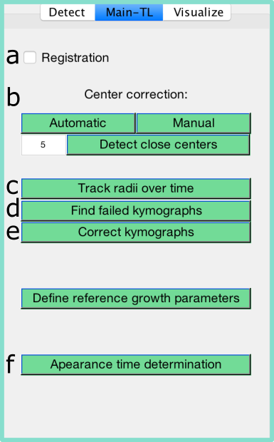
ColTapp can track the radius of detected colonies through time on time-lapse image series. First, all colonies need to be detected on the latest (or a late) frame in a time-lapse series. All time-lapse associated functions are accessible through a dedicated tab on the GUI. The buttons are labeled with letters and text on this page referring to buttons uses these letters.
ColTapp can correct for slight image drift occuring in time-lapse imaging. This process is called image registration. The correction is not applied to the images themselves but to the detected centers of each colony resulting in a center for each colony and frame. Therefore, it is important that all colonies of interest are already detected before the drift correction is enabled. Enable and disable the drift correction with the toggle a Registration. To improve speed of the registration calculation, the user is asked to draw a small rectangular area on the image which is subsequentially used to automatically detect image drift. It is suggested to select a part of the image which includes clear edges (e.g. border of an agar plate) and does not include any changing parts (e.g. colonies). If the registration should be re-calculated, the user can remove the stored registration vector via Options/ Main-TL tab/ Reset registration.
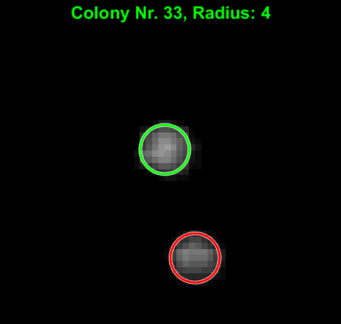
The centering of colony circles is crucial to track radii over time, especially at early timepoints when colonies are small. ColTapps includes automatic and manual center corrections executable with the buttons under b. Beforehand, it is strongly suggested to turn on Autoconstrast or, even better, Improve lighting which can be accessed in the Detect tab of the GUI. ColTapp offers an automatic center correction, by tentatively detecting circles on sub-images cropped from an early frame based on the location and radii of the colonies detected on the reference frame. These newly detected circles’ center coordinates are kept as colony center, unless they are farther away than a user-defined threshold from the original coordinates or if they are set to the center coordinates of another colony in close proximity. In these cases, the correction is skipped, and the colonies are added to a list for subsequent manual center correction. If no circle is detected at all because the colony is not yet visible at that timepoint, the same process is repeated 10 frames later. The user is able to monitor this process visually. The green circle is the one chosen by ColTapp as the correct center, red circles are discarded.
If the automatic center correction failed, manual center correction is available (b). The user is presented with cropped sub-images of each colony and can click manually on the correct center of each colony. Buttons to add the displayed colony to a list of colonies for which the center correction should be repeated 10 frames before or later are displayed. The colonies of these lists will be automatically displayed afterwards.
After all colonies are detected (and optionally the registration is enabled and center correction finished), radius tracking can be started with a simple click on the button c “Track radii over time”. This calculates kymographs for each colony from which radius growth curves are derived.
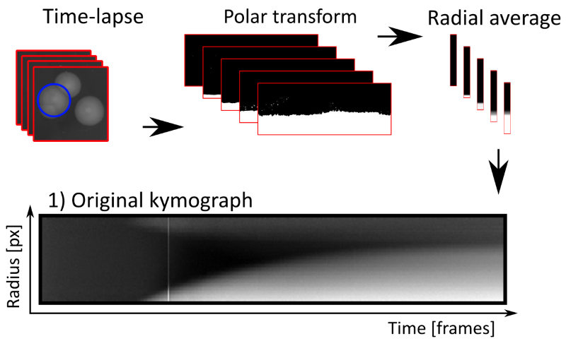
Neighboring colonies can be visible as blurry regions in the top of kymographs, hindering creation of clean binary images.
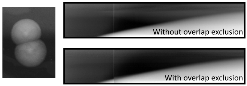
To reduce this phenomenon, before the kymograph creation process, overlapping colonies are automatically detected and the ranges of angles corresponding to adjacent colonies are discarded from the polar transformed intensity data. If more than 90% of all angles are discarded because of overlap, the exclusion of angles is omitted completely, to avoid reducing the available data too much. The overlap detection functionality can be deactivated or tuned with Scale radius for overlap (accessible in Options/TL-tab). This scaling factor is multiplied to the radius of the focal colony from which center neighboring colonies are tested for overlap: by increasing it, a user may choose to discard ranges of angles corresponding not only to overlapping colonies but also very close colonies. Note that this increase might lead to high proportions of angles to be discarded. Decreasing the scaling factor leads to reduced ranges of excluded angles. This might be useful in densely populated plates to still achieve some overlap exclusion to increase quality of kymographs at late timepoints.
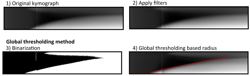
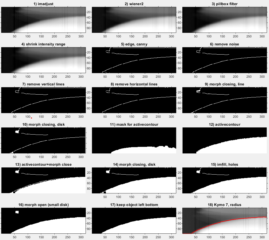
To derive the radial growth curve from kymographs, the edge of the colony is detected by finding the transition from white to black. ColTapp includes two methods to determine the growth curve: 1) Global thresholding and 2) Edge detection mode. Both methods first apply an automatic contrast enhancement function, then a pixel-wise adaptive low-pass Wiener filter followed by a circular averaging filter (pillbox) to the kymograph to derive a smoother image. Additionally, a low-pass threshold for maximal intensity may be applied. Global thresholding then transforms the grayscale kymograph into a binary image based on an automatically determined threshold (Otsu’s method). See below for methods to manually correct the threshold.
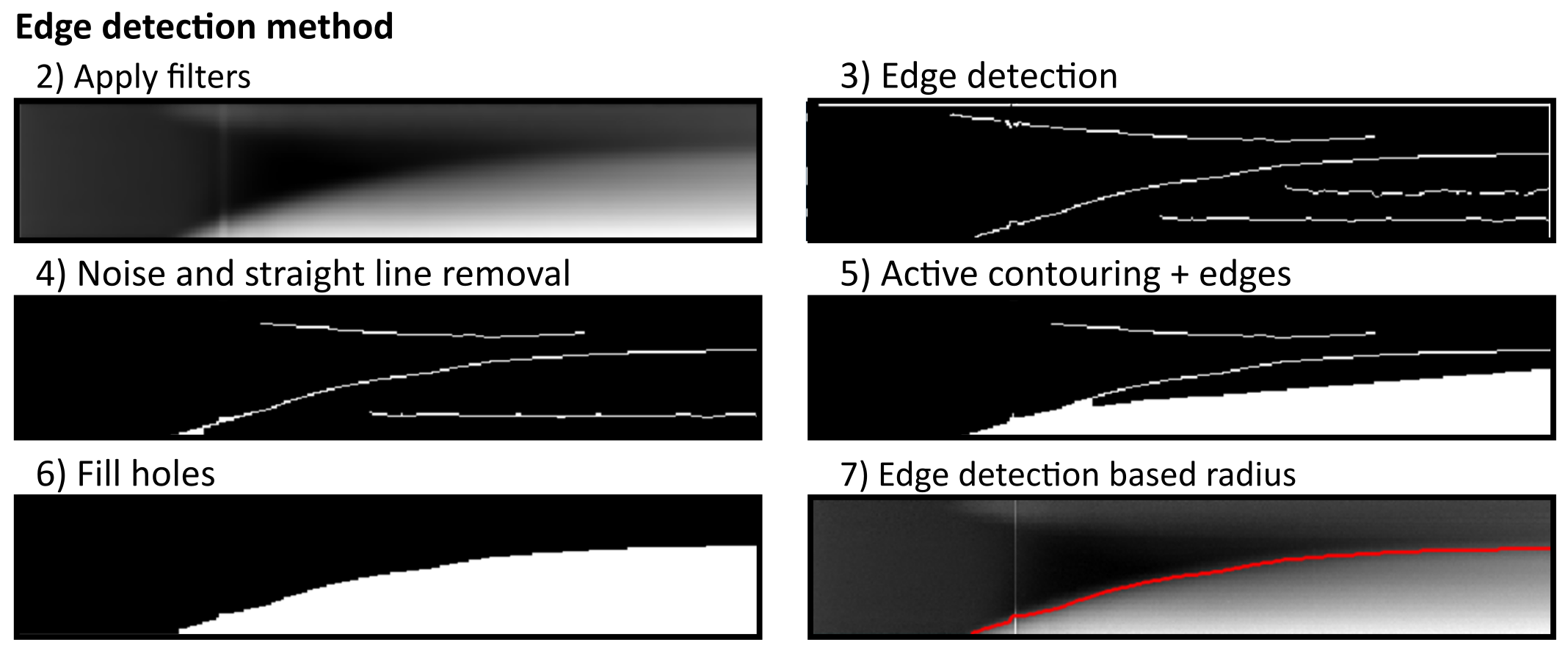
The Edge detection method uses a series of edge detection and morphological operations. In brief, the method by Canny is used for initial edge detection. Subsequently, small isolated foreground pixels are removed with area opening operations. Straight vertical and horizontal lines, typically originating from light artifacts and particles on the agar respectively, are removed. Two iterative morphological closing operations are used with line- and disk-shaped kernels, respectively. Additionally, active contouring using the Chan-Vese method is applied to the pre-processed kymograph to derive a second binary image with a filled region of probable colony area. The two binary images are merged, and morphological closing is performed to close potential gaps to successfully fill connected regions afterwards. A final morphological opening is applied to remove jagged edges. The fully connected object located in the lower right side of the kymograph (corresponds to end of time-lapse and close to colony center) is kept as the only foreground object in the binary image. See below for methods to manually correct and adjust each of the values corresponding to image manipulation steps.
ColTapp has an inbuilt function to automatically detect radial growth curves with probable errors derived from kymographs based on the number of local maxima, size of radius differences from frame to frame, monotonicity, and number of frames without a successful radius determination (button d Find failed kymographs). These (or any) radial growth curves can be manually corrected with a dedicated tool (button e Correct kymographs) which allows the user to switch for each colony individually between Global thresholding and Edge detection method, and adjust any parameter of the two methods to derive best parameter combinations to derive the radial growth curve from the kymograph. See below the seperate GUI layout, a table describing all parameters and the display provided by the ‘Show steps’ button.
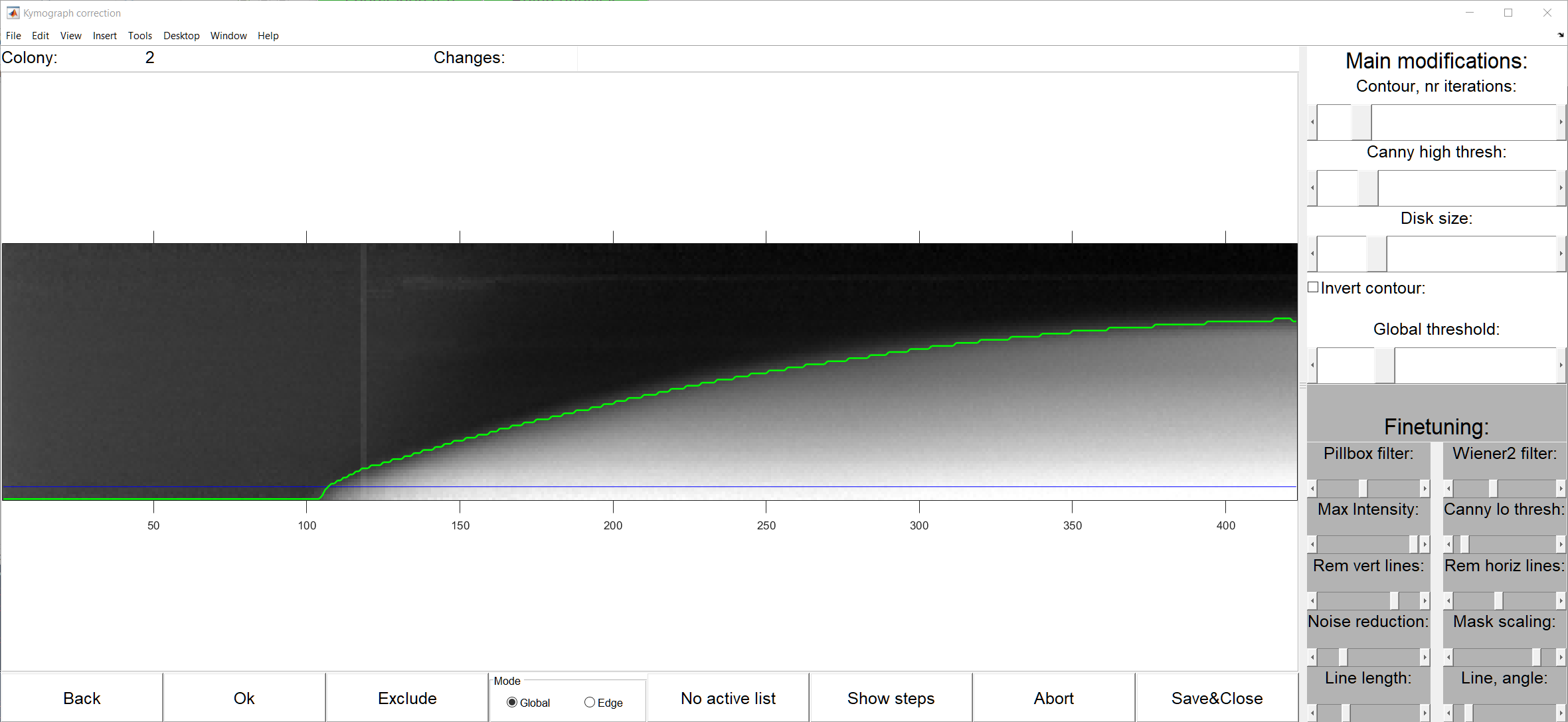
| Parameter | Mode | Function |
|---|---|---|
| Contour, nr iterations | Edge | Number of iterations for contouring. Lowering this value might reduce overshoot of radius calculation and increasing this value might help in even out jaggy radius determination |
| Canny high thresh | Edge | Threshold for initial edge detection. Only edges with a strength higher than this threshold are preserved. |
| Disk size | Edge | Disk size for various morphological operations. Higher values might help smooth out jagged radius detection but potentially introduce noise, especially close to the beginning of the colony growth |
| Invert contour | Edge | Sometimes, especially if colonies only fill out a small area of the kymograph, inverting the contour is needed |
| Global threshold | Global | This value defines an offset of the automatically defined (Otsu) binarization threshold |
| Pillbox filter | Both | Filtering strength. Higher values lead to smoother images but may introduce noise |
| Wiener2 filter | Both | Filtering strength. Higher values lead to smoother images but may introduce noise |
| Max Intensity | Both | Low-pass filter for intensity. Values higher than the set value are set |
| Canny lo thresh | Edge | Edges with a strength below than this threshold are discarded |
| Rem vert lines | Edge | Foreground pixels are discarded if a straight vertical line defined as number of white pixels per line is higher than this threshold |
| Rem horiz lines | Edge | Foreground pixels are discarded if a straight horizontal line defined as number of white pixels per line is higher than this threshold |
| Noise reduction | Edge | Scaling factor for small foreground object removal |
| Mask scaling | Edge | Scaling factor for initial mask creating for iterative contouring |
| Line length | Edge | Length in pixels of a line closing morphological operation |
| Line angle | Edge | Angle of a line closing morphological operation |
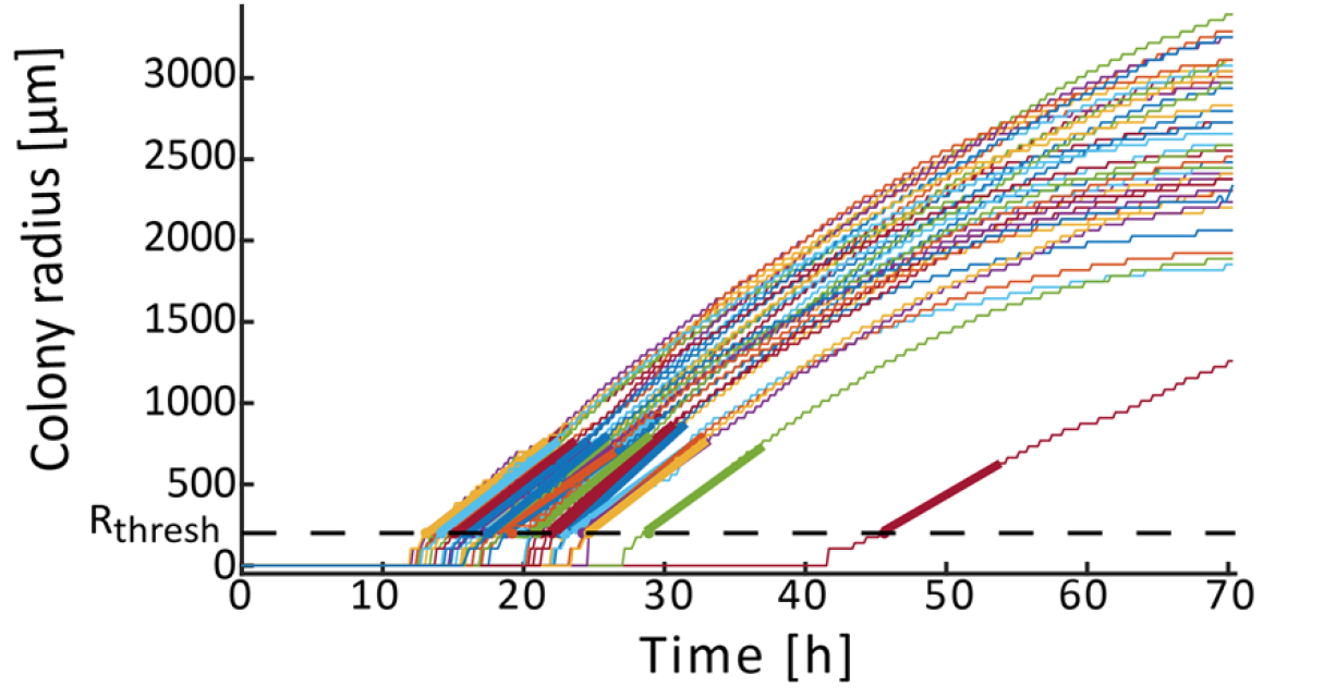
Once the colony radial growth curves defined, we can derive each colony appearance time and growth rate. We define a detectable size threshold in micrometers (Rthresh), and the time at which a colony reaches this threshold as the colony appearance time. The minimal possible Rthresh depends on the image quality and needs to be set at the same value for comparisons of tapp in different experiments. In our analysis setting, we assume that colonies reaching this size are already in the linear growth phase. Tracking the colony radius over time using time-lapse imaging makes it possible to directly determine colony appearance time and linear radial growth rate. ColTapp determines these parameters by detecting the first of 6 consecutive frames for which a colony radius is bigger than Rthresh (default: 200 μm). The following radius measurements within a user-specified number of frames (Frlin, default: 50 frames) are used for a linear regression (tick slopes in the following figure). Frlin might need to be reduced to only use a timespan in which radial growth is approximately linear. Additionally, Rthresh can be adjusted depending on the image resolution and bacterial species investigated. Both can be adjusted in the Options. The reason to perform a linear regression to determine tapp instead of simply observing the time when a colony radius reaches Rthresh is that it reduces artificial noise, to be expected if camera resolutions are low (for example if 1 pixel = 50 μm). Note that a low rate of image acquisition (long interval between time-lapse frames) might result in under-sampling.